A logical misalignment between our knowledge-based expectations and real-world observations manifests as a paradox. The natural world has its fair share of paradoxes. Below are five paradoxes in biology, along with their proposed resolutions. Several of these paradoxes create excitement, while some, unwittingly, were created out of excitement.
“How wonderful that we have met with a paradox. Now we have some hope of making progress.”
— Niels Bohr, theoretical physicist.
The C-value paradox
more genetic material ≠ more biological sophistication.
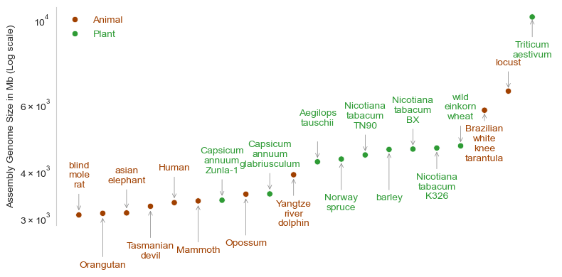
DNA is the blueprint of all living organisms and the more complex a life form is the more elaborate the blueprint will be. This seems rather intuitive. And, this is by and large true. Starting from single-celled organisms to higher life forms such as plants and animals, there is an increase in the genome size (that’s total DNA in a cell). However, there are prominent and persistent deviations from this pattern. We do see multiple cases where a seemingly simpler life form has larger genome size compared to organisms that show greater complexity. This observation is the basis of the C-value paradox. So, what’s C-value?
There was some debate in the literature about what is ‘C’ in C-value. However, it is now clear that C means constant - “the amount of DNA that was characteristic of a particular genotype” (reference).
The figure below shows the top ten largest genomes in animals and plants based on the data given over here. If we compare within animals, it is rather bizarre to see that a locust has more than double DNA than Humans! Why? Also, notice that all the plants in this figure have genome sizes greater than those of humans. What does these differences really mean? Maybe our knowledge that genome sizes increase with complexity was intrinsically flawed to begin with.
Show Python code
import pandas as pdimport seaborn as snsimport matplotlib.pyplot as pltimport numpy as npdf_genomes = pd.read_csv("https://raw.githubusercontent.com/wrf/genome-size/refs/heads/master/elliott2015_data/rstb20140331supp1.tab", sep="\t")df_genomes_grp = (df_genomes .groupby("Taxon Group", group_keys=True) .apply(lambda x: x.nlargest(10, 'Assembly Genome Size (Mb)'),include_groups=True) .sort_values("Assembly Genome Size (Mb)") .reset_index(drop=True) )df_plot = df_genomes_grp[df_genomes_grp["Taxon Group"].isin(["Animal","Plant"])]df_plot = df_plot.copy()df_plot["Label"] = df_plot["Common Name"].fillna(df_plot["Species"])df_plot["Label"] = df_plot["Label"].str.replace(" ", "\n")fig,ax=plt.subplots(figsize=(8,4))custom_palette = {'Animal': '#A04000', 'Plant': '#2E9B35'}scatter = sns.scatterplot(data=df_plot, x="Species", y="Assembly Genome Size (Mb)", hue="Taxon Group", palette=custom_palette)handles, labels = scatter.get_legend_handles_labels()group_color_map =dict(zip(labels[0:], [h.get_color() for h in handles[0:]]))for i, row in df_plot.iterrows(): group = row["Taxon Group"]# print(i)if(i%2==0):if(i>25): i=20 plt.annotate( row["Label"], # text label xy=(row["Species"], row["Assembly Genome Size (Mb)"]+50), # coordinates of the point xytext=(0, i*1.25), # offset for label position textcoords='offset points', ha='center', color=group_color_map.get(group, 'black'), arrowprops=dict(arrowstyle="->", lw=0.5, color='grey') # arrow style and color )else:if(i>22): i=20 plt.annotate( row["Label"], # text label xy=(row["Species"], row["Assembly Genome Size (Mb)"]-50), # coordinates of the point xytext=(0, -i*2.5), # offset for label position textcoords='offset points', ha='center', color=group_color_map.get(group, 'grey'), arrowprops=dict(arrowstyle="->", lw=0.5, color='grey') # arrow style and color )legend = ax.legend(ncol=1, loc='upper left', frameon=False)for text, handle inzip(legend.get_texts(), handles): text.set_color(handle.get_color())plt.yscale("log")sns.despine(bottom=True)ax.axes.get_xaxis().set_visible(False)ax.yaxis.grid(False)plt.tight_layout()plt.ylabel("Assembly Genome Size in Mb (Log scale)")#plt.savefig("genomes.png")plt.show()
A multitude of factors contribute to variations in genome sizes. In an organism, the entire genome never codes for functional proteins. In fact, a small fraction of the genome codes for proteins (in humans it’s about 2%). The remaining large fraction is required for regulation of the different processes involving DNA. Which means that a genome can increase in size without much increase in the perceived complexity of the organism. Here, complexity broadly refers to structural and functional capabilities of an organism. Also, as highlighted in this review, genomic features such as introns (non-coding region of mRNA), repeatomes (repeated sequences in the genome), polyploidy (presence of more than two sets of chromosomes), etc. can bloat the genome size without contributing much to the overall complexity of the organism.
Levinthal’s paradox
A Biochem101 staple.
Proteins must adopt a specific three-dimensional structure to perform their function. How a given polypeptide chain folds into a specific conformation has baffled researchers across different disciplines. The perplexity stems not just in terms of adopting a (meta-) stable conformation but also, and even more provocatively, from the speed at which a particular folded state is achieved within the cell. Typically, folding of a protein takes a few milliseconds. Exceptionally, there are reports of some protein folding in microseconds and in a few seconds as well. Now if we consider, theoretically, the different conformations a polypeptide can adopt we’ll get an extremely large number of possibilities. And, from these options narrowing done to one specific confirmation that too within milliseconds is indeed a daunting task.
In his 1969 paper, Cyrus Levinthal presented a conceptual argument that if a small protein (having 150 amino acids) has to sample all possible confirmation before arriving at an energetically stable conformation, the total time required for that process would be more than the age of the Universe. Based on his thought experiment, he proposed that the process of protein folding must not involve exhaustive sampling of the entire conformational space. Rather, verbatim, “We feel that protein folding is speeded and guided by the rapid formation of local interactions which then determine the further folding of the polypeptide.” Curiously, there was no use of the word paradox in this article. More than two decades later, researchers at NIH, presented a mathematical framework to explain how proteins can adopt a functional folded state at biologically relevant timescales. They chose a two-word title for their article - Levinthal’s paradox - and rest, as they say, is history. Since then, this paradox, which started as a thought experiment, has captivated researchers and has sparked juicy conversations and vivid analogies (e.g., by Richard Dawkins in The Blind Watchmaker - albeit in a different context).
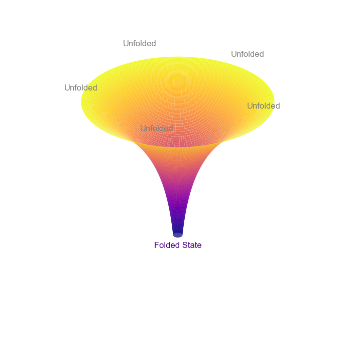
It is now well-established that protein folding does not proceed by randomly testing all possible conformations. Over the years, multiple proposals have been made to explain the reduced folding time. For instance, the nucleation-growth model suggests that the initial formation of structured regions (folding nuclei) guides the protein to an energetically stable conformation. And, the diffusion-collision model assumes that the secondary structure elements (microdomains) forms independently along the polypeptide chain which then combine to form the native structure. Similarly, there are some additional well-studied hypotheses to understand protein folding. It is important to note that these models are not mutually exclusive and can act synergistically to speed-up the folding process. A unified view of protein folding is represented by the “folding funnel”. Here, different unfolded states can follow multiple folding pathways to form a stable folded conformation (as shown in the schematic diagram below).
Show Python code
import numpy as npimport matplotlib.pyplot as pltfrom mpl_toolkits.mplot3d import Axes3Dr_max =2r = np.linspace(0.1, r_max, 100)theta = np.linspace(0, 2* np.pi, 100)R, T = np.meshgrid(r, theta)Z = np.log(R)X = R * np.cos(T)Y = R * np.sin(T)fig = plt.figure(figsize=(10, 7))ax = fig.add_subplot(111, projection='3d')# Plot the funnelax.plot_surface(X, Y, Z, cmap='plasma', edgecolor='none', rstride=1, cstride=1, antialiased=True)num_labels =5angles = np.linspace(0, 2* np.pi, num_labels, endpoint=False)for angle in angles: x = r_max * np.cos(angle) y = r_max * np.sin(angle) z = np.log(r_max) +0.3# Add label ax.text(x, y, z, "Unfolded", color='grey', fontsize=12, ha='center')ax.text(0, 0, np.log(0.1) -0.3, "Folded State", color='indigo', fontsize=12, ha='center')ax.set_axis_off()plt.tight_layout()plt.show()
Peto’s paradox
Spoiler alert - it is no longer a paradox!
Mutations can occur spontaneously in all dividing cells and there is nothing particularly extraordinary about this phenomena since all cellular processes are error-prone. Sometimes these mutations can result in loss of control of cell division which is a hallmark of cancer. So, it seems rather intuitive that more a cell divides more are the chances of getting cancer-causing mutation. Further, the more the number of cells an organism has the greater are the chances of accumulating such mutations. These facts imply that larger (more cells) and long-living (more cell divisions) animals should be more susceptible to cancer than smaller and short-lived animals.
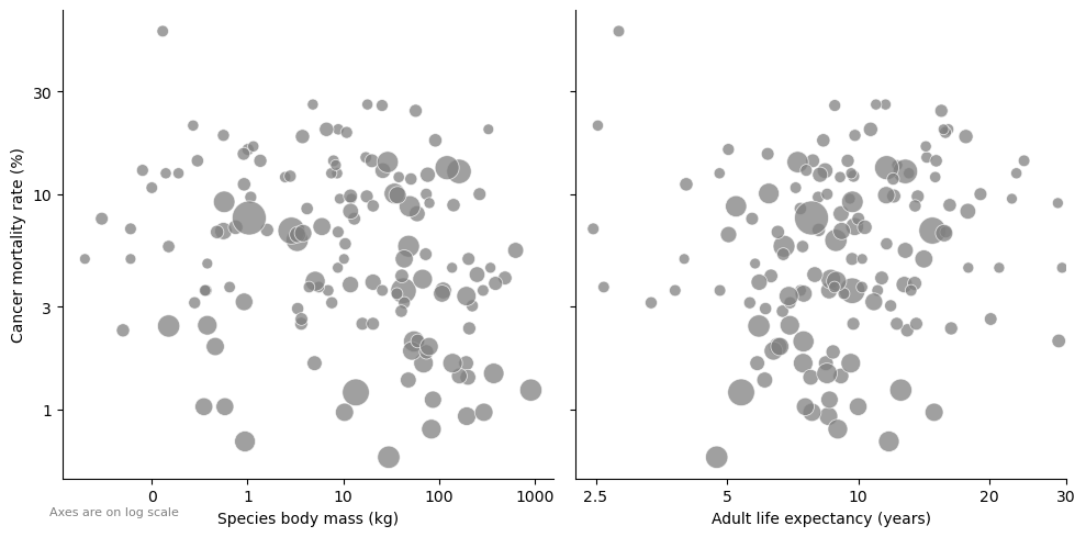
In 1977, Richard Peto, showed that there is no correlation between size, longevity and cancer across species. This observation is popularly known as Peto’s paradox since it apparently contradicts with the arguments made above about chances of more mutations (cancer) with size and longevity. There are some prominent examples supporting Peto’s paradox e.g., asian elephants, despite their large body size, have lower prevalence of cancer compared to humans. Myotis pilosus (Rickett’s big-footed bat) has a much longer life-span compared to humans (after adjusting for body-size) and still has lower cancer prevalence. Active research in this area has established reasons for this conundrum. Elephants have ~20 copies of the TP53 gene while humans have only one. This gene is one of the extensively studied tumor suppressor genes that prevents development of cancer. Similarly, bats show lower levels of gene products that are known to promote cancer growth.
The figure below is adapted from the data for Figure 3 in this article, where the authors conclude that “cancer mortality risk is largely independent of both body mass and adult life expectancy across species”.
Show Python code
import pandas as pdimport numpy as npimport matplotlib.pyplot as pltimport matplotlib.ticker as mtickerimport seaborn as sns# https://github.com/OrsolyaVincze/VinczeEtal2021Nature/blob/main/SupplementaryData.xlsdf2 = pd.read_csv("SupplementaryData.csv")df2 = df2[df2["CMR"]!=0]df2["CMR"] = df2["CMR"]*100df2["Adult life expectancy"] = df2["Adult life expectancy"]/365df_long = pd.melt(df2, id_vars=['CMR','No. individuals with available postmortem pathological records'], value_vars=['Species body mass (kg)', 'Adult life expectancy'], var_name='Variable', value_name='Value')g = sns.FacetGrid(df_long, col="Variable", height=5, aspect=1, sharex=False)g.map_dataframe(sns.scatterplot, x="Value", y="CMR", alpha=0.75, color="gray", size="No. individuals with available postmortem pathological records", sizes=(50, 500))for ax, title inzip(g.axes.flat, g.col_names): ax.set_xlabel(title) ax.set_xscale("log") ax.set_yscale("log") ax.set_yticks([1,3,10,30]) ax.set_yticklabels(["1","3", "10", "30"]) ax.xaxis.set_major_formatter(mticker.ScalarFormatter()) ax.xaxis.set_minor_locator(mticker.NullLocator()) ax.yaxis.set_minor_locator(mticker.NullLocator())if("life"in title): title = title+" (years)" ax.set_xlabel(title) ax.set_xticks([2.5,5, 10, 20,30]) # Set tick positions ax.set_xticklabels(["2.5","5", "10", "20","30"]) ax.set_xlim(2.25,30)g.set_titles("") g.fig.text(0.05, 0.05, "Axes are on log scale", ha='left', fontsize=8, color='gray')g.set_ylabels("Cancer mortality rate (%)")plt.tight_layout()plt.show()
Small wonder, Peto’s paradox ignites interdisciplinary discourse spanning domains like ecology, evolution, and oncology. However, earlier this year, researchers in the UK used a Bayesian phylogenetic framework to test Peto’s paradox and concluded: “Larger species do, in fact, face higher cancer prevalence than their smaller counterparts.”
The lek paradox
Sexual selection vs Natural selection.
In the Darwin’s theory of evolution, natural selection plays a central role in the selection of genetic traits. There is another important factor that contributes to selection of traits and that is sexual selection. In sexually reproducing animals mate preference can strongly influence the selection of specific traits and at times such selection might seem counter-intuitive when looked at from the lens of natural selection. A case in point is the peacock’s train – based on natural selection principles it should not be long because of the greater risk of exposure to predators. On the contrary, we do see elaborate trains with splendid eyes because it absolutely ensures mating, so it’s worth the risk!
There are in fact diverse ways in which sexual selection manifests in different species and one such set-up is lek mating system. A gathering of males to competitively display physical traits to attract a female is known as lekking. The display can involve traits like size, vocal skills, acrobatic abilities, etc. The females visit lekking sites not for any long-term relationship or parenting commitment but for just one thing – sperms. Expectedly, all females want it from the best male. This results in a few males disproportionately fathering a large number of offspring. So, in a Lek system, given the strong female preference for a trait, the genetic diversity in a particular trait will tend to deplete since there is no reason to tinker with that trait. However, we do see genetic diversity in sexually selected traits — the Lek paradox.
Multiple hypotheses have been proposed to resolve this paradox such as the ‘genic capture hypothesis’, where the development of the sexually selected traits is based on the conditions (biotic and abiotic) and the response to conditions is polygenic. Now the question is - what do we mean by condition? As referred here, it is “the pool from which resources are allocated” i.e. condition corresponds to “residual reproductive value” in traditional life history models, and accounts for a large proportion of fitness.
Simply put, it is hard to “fix” a trait because widespread genetic variations underpin the development of secondary-sexual traits. The Lek mating system is indeed fascinating because when a female selects the best male, she is naturally selecting overall “good-genes”.
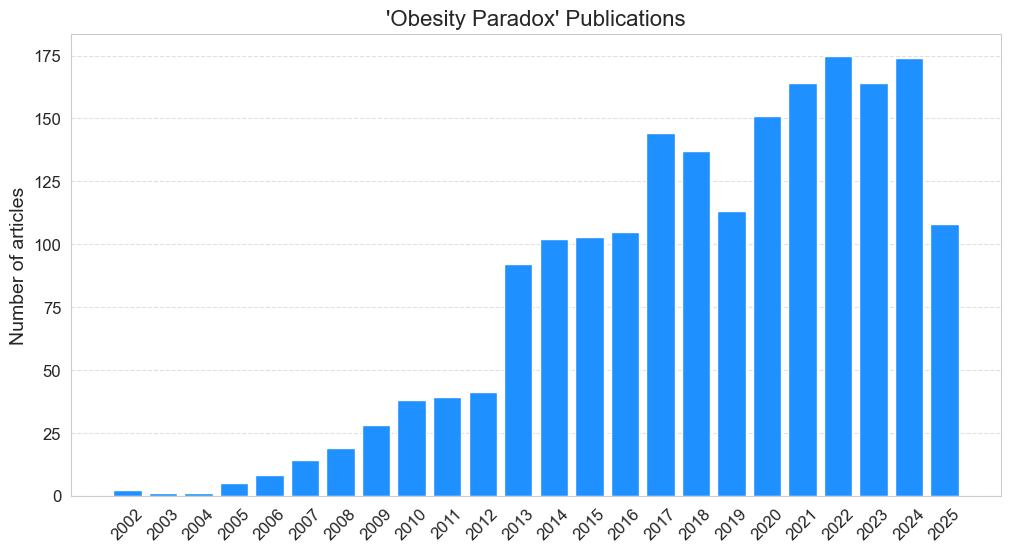
Obesity has reached epidemic proportions with some serious public health implications. It directly contributes to the development of several chronic diseases like type 2 diabetes, cardiovascular diseases, and certain cancers, etc. There are no benefits to being obese. In 1980, R Andres reported that the Body Mass Index (BMI) that leads to lowest mortality tends to increase with age. This work laid the foundation for what we now know as the obesity paradox since it questioned the “beautiful hypothesis” that increasing weight is associated with increasing mortality. In early 2000’s retrospective meta-analyses by researchers from top institutions such as Cleveland Clinic, Harvard Medical School etc. endorsed this paradox. These observations, which are misleading at best and dangerous at worst, spread like wildfire in popular media such as Time and The Guardian. Till date, there are about 2,000 articles in PubMed, as shown in the timeline below, having “obesity paradox” in title or abstract.
Show Python code
from Bio import Entrezimport matplotlib.pyplot as pltimport matplotlib.cm as cmfrom collections import CounterEntrez.email ='example@test.com'#change email idpubs_diab = Entrez.esearch(db="pubmed", term="('obesity paradox'[Title/Abstract])",\ retmode="xml", retmax=9999) record = Entrez.read(pubs_diab)pubs_diab.close()idlist = record["IdList"]handle = Entrez.efetch(db="pubmed", id=",".join(idlist), retmode="xml")records = Entrez.read(handle)handle.close()# Extract publication yearsyears = []for article in records["PubmedArticle"]: pub_date = article["MedlineCitation"]["Article"]["Journal"]["JournalIssue"]["PubDate"]if"Year"in pub_date: years.append(pub_date["Year"])year_counts = Counter(years)years_sorted =sorted(year_counts.keys())counts = [year_counts[year] for year in years_sorted]fig,ax = plt.subplots(figsize=(12,6))plt.bar(years_sorted, counts, color='dodgerblue')plt.ylabel("Number of articles", fontsize=14)plt.title("'Obesity Paradox' Publications", fontsize=16)plt.xticks(rotation=45, fontsize=12)plt.yticks(fontsize=12)plt.grid(axis="y", linestyle="--", alpha=0.6)plt.grid(axis="x", linestyle="none")plt.show()
An editorial in Nature gives an eloquent background to this paradox and argues against it by delineating various biases – such as misclassification bias, reverse causation, and collider stratification bias – that could have influenced the interpretation of the data relevant to this paradox. A rather funny anecdote about this paradox is that when researchers observed cases that go against this paradox then, instead of using this as an evidence to refute the paradox, they chose to present it as “paradox within a paradox”. The hullabaloo over the obesity paradox is a reminder to exercise critical thinking faculties when interpreting data, particularly when it has profound public health implications
The fundamental issue with the genesis of the obesity paradox lies in the way obesity is defined based on BMI. This definition misses vital details such as the distribution of body fat, differentiation between lean muscle and fat mass, and aging related decrease in muscle mass with increase in body fat.
A commission of 58 researchers from across the globe, earlier this year proposed a new definition and diagnostic criteria for obesity which focuses on how excess body fat (adiposity) affects the body. They classified obesity into two categories - preclinical obesity, when there is excess adiposity but the organs function normally, and clinical obesity, characterized by dysfunctioning of tissues and organs due to excess adiposity.